Debugging in MARS

This is a topic that is kind of difficult to effectively teach on paper, but I'm going to go ahead and try my best.  The ability to debug your code in MARS is perhaps its most important feature, and it would be a shame if I were not to include a post on this on my blog.  Further, it is pretty inescapable - you will have to use it at some point whether you like it or not, otherwise you'll get stuck.  If you are/were anything like me in my freshman to sophomore years, you'd groan any time you'd have to reach for the debugger - fortunately, this debugger is pretty well designed and its functionality maps intuitively to how MIPS is executed.

Let me set the scene first:

I have this short program with a bug in it.  You might see it offhand, but the goal here is not to simulate a realistic scenario - instead it is to walk you through the process of fixing it.  Assume I have no idea what the problem is, and I'm completely baffled as to why I have an infinite loop here.  I've read over my code about ten times, and I can't find anything wrong.  Time to bring out the debugger.

When you build your program, you are automatically taken to the execution tab.  You will see something like this in the text segment of the screen:

This is your final program as the assembler built it.  All pseudo-instructions have been translated to real instructions, and we're looking at an interpretation of the machine code that was generated.  This is what MARS will run when we hit the play button.

The leftmost column is the breakpoint column.  A breakpoint is sort of an intervention into the running of your program that causes the machine to pause so that you can look at its state.  You can tell MARS to place a breakpoint at any line - just click the box to enable a breakpoint at that location.

The second column is the address column.  Most of the time you can ignore this column completely, but there may be times that you want to compare the contents of the $ra register to where you expected the program to jump to.  It just states where the binary instruction is located in memory when the program is running.

The third column shows you how your instructions are represented in binary.  I can't think of a situation where this would be all that useful unless you were writing the MIPS virtual machine yourself, which you're probably not planning on doing if you're using MARS.

The basic column shows you the instruction in assembly form, rather than binary form.  This is how you tell what part of your code you're looking at, in conjunction with the unnamed rightmost column, which tells you the line number in your assembly file that the instruction comes from and any comments you may have added.

You may notice that the labels factorial and exit are entirely absent.  This is somewhat unfortunate because you will usually want to set a breakpoint immediately following those labels.  The solution is just to put a comment that you can recognize on the first line underneath the label next to an instruction.  Lines that only contain comments won't show up at all.  I can tell that line 8 is where the factorial loop begins, because that's the instruction that exits the loop and I always put that instruction at the top.  You may prefer some other style whereby the first instruction in your loop does not look like this, but you'll recognize where a section starts with practice.

Since I have an infinite loop, I'm going to go ahead and put a breakpoint right at the top of that loop:

I can now hit the play button to run the program.  Lo and behold, my program pauses at the top of the loop:

I can tell where the program has stopped because that line is highlighted in yellow.

Now that the program has paused itself, I have several options.  I can run the program line by line on my command, I can run it really slowly, or I can keep pressing play and running into my breakpoint and just observe the machine's state once every time the loop cycles.  For the first option, I can use two of the buttons on the toolbar:

The third button from the left will move the machine's state forward one instruction, and the fourth will move the machines state backward one instruction (it will return to the previous state).  I can keep hitting this button until something looks off.

I could also play with the slider next to the toolbar:

By default this is set to the max setting, which just tells MARS to run the program as fast as possible (as fast as your computer can run it).  If I move the slider to the left, I can choose a specific number of instructions per second in the range of 1 - 30:

There's a bit of a quirk that can show up sometimes with this feature.  If you ever move the slider back to the right after changing its setting, MARS may end up running your program in slow motion anyway.  This is hardware dependent and happens only to some people.  If you run into this problem, just save your file and restart MARS.

For the third technique, all I have to do is keep pressing play and MARS will hit my breakpoint again, having gone through the loop one more time.  In this specific case, I prefer to use this tactic.

No matter which technique you decide is most user-friendly, you will have to say hello to the registers panel on the right side of your screen:

There are three tabs here but Coproc 1 and Coproc 0 are for advanced use only, so we'll stick to the Registers tab.  You have the whole family of registers at your disposal here.  In the case of this program, I was using $t0, $t1, and $t2, so I'll want to look at those.  Right now they contain the initial values that I gave them before the start of the loop, because MARS hasn't actually simulated one loop cycle yet.  If I hit the play button, the MARS will hit my breakpoint again and I'll see this:

The register that was last written to is highlighted in green.  Notice that the values stored in these registers still hasn't changed, despite having gone through one loop cycle.  That's not the expected behavior - I should see that the counter has been incremented, but it hasn't.  Hmm.

Oh!  I forgot to increment the counter!  Doy.

I added my increment at line 11, and the program is fixed!  Yay!

There is one more important feature that I didn't need to use, though.  My little program doesn't go to memory.  Sometimes I might want to look at memory, since the state of my program is dependent on it.  There is a screen for this underneath the breakpoint setting screen:

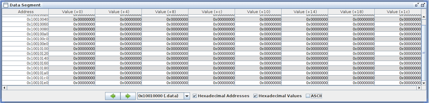
This shows you the entirety of main memory.  Every single byte.  The left column tells you the address in memory that the row begins at.  From left to right, the columns next to this one show the contents of several words in increasing address.  The column labels of these columns tell you the offset of each word from the address all the way to the left.  You will have to be familiar with endianness if you are looking for resolution at the byte level.  For integers in MIPS, the bigger bytes are placed first, so it looks exactly as you would write the integer on paper, but in hex.  You can toggle the hex off if you'd like with the convenient checkbox at the bottom, though.

Also useful is the drop-down menu that will allow you to travel between different areas in memory.  Because main memory is so big, this allows you to skip the process of scrolling down thousands of times.  Most of the time we're interested in the contents in the .data section, which is the default location anyway.

Like the registers tab, the word that was last written to will be highlighted while debugging:

In this case I've just written the word 15 to address 0x10010000.

And that's it.  If you have any questions or are running into trouble in ways that this tutorial hasn't addressed, feel free to leave a comment.  I will be checking my blog often, and will update this post with attribution if you run into an interesting problem.

MIPS: Millions of Instructions Per Second (Part 4)

In the last post I talked about functions and register conventions in MIPS.  I will continue the topic of functions in the next and final part, but we'll take a break from that and discuss bitwise operations and files.

 

Bitwise Operations

 

In MIPS and in most processor architectures, memory is byte-addressed.  Every byte is given its own number as a reference for accessing it.  But a byte consists of 8 bits.  This means that none of those bits have an explicit address, even though we may sometimes want to look at one bit individually.  To get around this problem, we can use bitwise operations.

MIPS provides the instructions and, or, xor, and nor, and their immediate counterparts.  You should be familiar with how these operations work on single-bit inputs.  On 32-bit registers, these instructions run 32 operations in parallel, one on each of the bits in the register.  So with two inputs, the far right bit of the first input is matched with the far right bit of the second input and put through the gate to get the result for the far right bit of the output.

For example, if we were to AND two 8-bit inputs:

All bitwise operations work on this simple principle.  There are uses for bitwise operations that come up a lot - let's go over those uses.

 

Isolating Bits With AND

 

This one is derived directly from the picture above.  There may be times when you want to observe a specific bit in a register, or a collection of bits - the simplest way to do this is to use andi with ones in the bit positions that you're looking at.  We will be using hex in our code - if you're not able to do the conversions in your head, I recommend practice but you may also use a calculator such as this one.

For example, if I want the lower 16 bits of a register, I can do this:

Anding with zeros sets the higher 16 bits to zero, while anding with ones ensures the lower 16 bits are kept the same.  This is equivalent to the following Java code:

Usually this sort of thing is done when dealing with bitfields, where each bit is a distinct boolean representing some condition.  Getting a nonzero result means the bit you're looking for is set, which means the condition is true.

Setting Bits With OR

On the other hand, you might want to write certain bits instead of reading them.  You can use the ori instruction to do this:

This will set the second bit from the right to one, and keep all other bits the same.  Usually this tactic is used in regards to bitfields as well, but in code that is setting conditions rather than checking for them.  This is equivalent to the following Java code:

Canceling Bits With AND

This is the opposite of the above - instead of setting a bit to one, you might want to set it to zero and keep all other bits the same.  You use andi for this too:

This sets the second bit from the right to zero, and is equivalent to:

Flipping Bits With XOR

Sometimes you just want to set certain bits to the opposite of what they are currently, regardless of what value they have.  For this, you can use xori with ones in the positions you want to flip:

This will flip the 13th bit from the right, while keeping all others the same, and is equivalent to:

And that's really it for bitwise operations.  They're pretty simple as long as you're able to do the binary to hex conversion.  Now let's move on to files.

 

Files

Java has abstractions for file operations that MIPS does not.  Instead of an object, each open file is given a number that we call its file descriptor.  All operations on that file will refer to this number so that we know we're dealing with it and not some other file.  If you've dealt with files in C, it is the same system just without the high-level code to simplify things.

All operations are done with syscalls.  Below is a table of the syscalls we'll be using:

Obviously the file has to be opened before we do anything with it.  Syscall 13 takes three arguments - the filename, a flag argument, and a mode.  Counter-intuitively, the "mode" in the traditional sense (read-only, write-only, etc) is sent through the flag argument, and mode is ignored entirely.  This usage is defined by the MARS environment, and may be different for other systems.  If we just want to read an existing file, we pass 0 for the flag.  For write-only mode, pass 1.  For write-only mode with automatic creation, pass 9.

The code below opens a file and prints its file descriptor:

MARS will assign file descriptors starting from 3, because 0, 1, and 2 are reserved for stdin, stdout, and stderr.  If your file is found, then 3 should be printed to the console.  If it isn't found, -1 will be printed instead.  The working directory for MARS is different depending on the operating system you're running it on - on Windows and Mac OS X, the working directory is the directory that the MARS jar is located.  On linux, the working directory is your home directory.

You can now use this file descriptor on the other three syscalls.  We can't write to the file because we've given 0 (read-only) for the flag argument, but we can read.  Syscall 14 accepts the file descriptor as its first argument, then the address of an input buffer to store the read data, then the number of bytes to read.  We need to set aside some space for the buffer in the .data section of our code in order to read:

$v0 will contain the number of characters read from the file.  If there are more than 16 left, it will read all 16 in this case.  If there are less, it will read however many bytes are left.  If it is already at the end of file, it will set $v0 to 0.  If there is an error, it will set $v0 to -1 or some other negative value.

There is no distinction between binary mode and text mode here.  If the data in the file is stored in ASCII, then it will load the ASCII data as is.  If it's not, it will load whatever else is in there in binary form and store it as is.  If we are dealing with an ASCII file and we print out the buffer as if it were a string...

...we will see the first 16 characters of its contents (also note that I forgot to use syscall 10 - don't do that).

Syscall 15 for writing is the same thing, just in the reverse direction.  It will read your buffer and write it to the file.  You can use flag 1 to write/replace, or you can use flag 9 to create a new file and write to it:

Since I use linux, the file showed up in my home directory and contained the string "this_buffer."

Finally, close the file using syscall 16:

This code just opens and immediately closes the file, but closing the file always works the same way.  Just put the file descriptor in $a0 and run the syscall.

To Be Continued

There's one last part!  Next time I'll be talking about recursion and the frame pointer.

Big-O Notation

Welcome to the start of a series of posts on algorithms.  This series will be mostly theoretical and does not require the knowledge of a specific programming language, operating system, or whatever else is necessary for learning other areas of computer science.  A class on algorithms usually has the distinction of being exceptionally mathematical, so you will need to know basic calculus (derivatives / integrals) and some discrete mathematics (summations).  I will be using Python to write code excerpts, but all you will really need to recognize is the logic in them.

Many students consider theory their weak point, but I will be writing most of the material in plain English.  I will point out the meaning of every symbol and mathematical operation the first time I use them.  The point of this series is to make the topic more approachable and avoid the confusion of formality.

Without further ado, algorithms.

 

What is an Algorithm?

 

An algorithm is a technique to solve a problem that can be represented mathematically.  It is not necessarily executed on a computer - in fact, we execute many algorithms in our heads every day.  Remember back in elementary school when you learned how to add two numbers together?  That's an algorithm.  So is long division, or whatever technique you learned to subtract.  Most algorithms that humans execute are basic and involve few inputs, but algorithms can be used to solve much more complex problems with millions to billions (to trillions (to quadrillions, etc)) of inputs.

When designing an algorithm, there are two primary goals in mind - correctness and efficiency.  Correctness is the most important property of an algorithm.  If it isn't correct, then what good is it?  A wrong answer computed instantly is no better than a right answer computed in infinite time.  Of course, a right answer computed instantly is infinitely better than a right answer computed in infinite time.  Efficiency is the second most important goal, and it is what most of the effort spent on algorithm design is after.  An algorithm can be efficient in respect to multiple quantities, but most often in respect to time and space.

When talking about the efficiency of an algorithm, we say that the quantity we are analyzing changes in respect to the size of the input.  A sorting algorithm will take longer to complete on a large array than on a small array because of the increased number of comparisons it has to perform.  It also requires more space to store a larger array.  It is usually the case that the running time of an algorithm and the amount of space it uses is strictly increasing with bigger input sizes.  Because of the increasing demand for computing resources, computer scientists will go out of their way to get every drop of efficiency out of their algorithms, granted that efficiency remains relevant at scale.

 

Asymptotic Growth

 

It is entirely possible to analyze the precise number of operations an algorithm takes to complete, but often it is unnecessary to relay every detail to other computer scientists.  Instead, it is common practice to describe an algorithm using a small set of basic functions that each grow faster than each other.  There are multiple ways of doing this, but the most frequently used is Big O Notation.

Take some function, f(n), and some other function, g(n).  We say that f(n) = O(g(n)) if, for some constant c and some threshold n₀:

$$f(n) \le c * g(n) \: \forall \: n > n_0$$

What does this mean?  It means that f(n) can be classified as O(g(n)) if g(n) is always bigger or equal to f(n) past some n.  In other words, f(n) grows just as fast or more slowly than g(n).  To clarify, the upside down A is just a fancy way of saying "for all."  You might be thinking: Can't I just make c really big, causing g(n) to become bigger than f(n)?  Well, no.  Because if f(n) is growing faster than g(n), then you can always choose a bigger n₀ to undo all that work that c is doing.

Take, for instance, the function f(n) = n + n².  Can we set g(n) = n, such that f(n) = O(g(n))?  If we set c to 1, then f(n) is only less than or equal to g(n) when n = 0.  Beyond that, f(n) is bigger.  Okay, how about setting c to 10?  f(n) becomes bigger when n = 3.  How about 100?  1000? 1,000,000?  There will always be some n such that f(n) overcomes g(n).  So we can't say that f(n) is O(g(n)).

Okay, well what about g(n) = 2n?  Nope, that won't work either.  That's the same thing as setting c to 2.  We have to multiply the original g(n) by something that grows with the size of the input, otherwise all we're doing is changing c.  We can multiply by any function of n that will enable g(n) to grow faster than f(n).  Since there's an n² in there, how about setting g(n) = n²?

If we set c to 1, it is clear that f(n) will remain above g(n).  But if we set it to 2, then that's equivalent to g(n) = n² + n².  Clearly, the left hand side of the addition will overcome the n term in f(n), so f(n) = O(g(n)).  Finally.

So what's happening here?  In one simple figure, this:

Setting g(n) = n² and c = 1 produces a function that will always be less than f(n) by n.  By setting c = 2, we produce a function that is always above f(n) past some point.  We can say that f(n) = O(n²) - we don't have to put the 2 in there, because c is just used in the proof.  In fact, putting the 2 in there doesn't really say anything about asymptotic growth, because...

...f(n) and g(n) are practically the same thing anyway.  This is what Big O Notation is actually saying, for the most part.  We could have also chosen g(n) = n³, or g(n) = n⁴ - both are an upper bound on f(n).  It just so happens that we found a function that perfectly describes f(n), which is also considered an upper bound on f(n).  If a function perfectly describes the asymptotic growth of another function, then it is necessarily true that one is Big O of the other.

It is fairly easy to prove that f(n) is O(g(n)) when it is actually the case.  All you have to choose is some c and some n₀, and then show that the two functions cross (possibly at n = 0), such that g(n) becomes greater than f(n) with increasing n.  In fact, we could have avoided all this trouble and just picked out the biggest term in f(n) and removed any multiplied constant from that term (in this case there wasn't one).  That's usually how computer scientists choose g(n), because it becomes second nature to be able to point out the fastest growing term.

But what if we have to prove that f(n) is not g(n)?  When I set g(n) = n, I never actually proved that it didn't work, I just explained away that no constant would be acceptable.  In a formal setting (like a midterm), we have to show that there really is no c that will work.  There's one way of doing this that will work pretty much all the time and is convincing, but it involves L'Hospital's rule.  If the following is true:

$$\lim_{n \rightarrow a} {f(n) \over g(n)} = {0 \over 0} \: \wedge \: lim_{n \rightarrow a} {f(n) \over g(n)} = {\pm \infty \over \pm \infty}$$

Then:

$$\lim_{n \rightarrow a} {f(n) \over g(n)} = {f'(n) \over g'(n)}$$

Which is to say, if the limit as n approaches a for both functions is zero or that same limit goes to positive or negative infinity for both functions, then you can divide one function by the other and take the derivative of both to get the same limit.  For analysis of algorithms, we're always interested in setting a to infinity.

What we can do is divide one function by the other and keep taking the derivative until all reference to n disappears in either the numerator or the denominator.  If this happens for f(n) first, then f(n) = O(g(n)).  If this happens for g(n) first, then f(n) =/= O(g(n)).  If both disappear at the same time, then f(n) = O(g(n)) as well.  If we try this technique with f(n) = n + n² and g(n) = n, then:

$$\lim_{n \rightarrow \infty} {f(n) \over g(n)} = {n + n^2 \over n} = {1 + 2n \over 1}$$

Because f(n) dominates g(n), f(n) =/= O(g(n)).  But setting g(n) = n² will work:

$$\lim_{n \rightarrow \infty} {f(n) \over g(n)} = {n + n^2 \over n^2} = {1 + 2n \over 2n} = {2 \over 2}$$

Setting g(n) = n³ will also work:

$$\lim_{n \rightarrow \infty} {f(n) \over g(n)} = {n + n^2 \over n^3} = {1 + 2n \over 3n^2} = {2 \over 6n}$$

You can use this method to prove either case, as long as both of the derivatives go to infinity at every step.  If they don't, then you'll have to try and use algebra to get around the problem.

 

Common Functions

 

You can use any g(n) that you want as an upper bound, but most of the time the appropriate g(n) will be one from a list of common functions with increasing growth rates:

1. O(1), also called constant.
2. O(log(n)), also called logarithmic.
3. O(n), also called linear.
4. O(n log(n)), also called linearithmic or loglinear.
5. O(n^c), also called polynomial.  If c = 2, quadratic.  If c = 3, cubic.
6. O(cⁿ), also called exponential.  The most common base is 2, but c can be anything.
7. O(n!), also called factorial.

It is standard to leave out the base when dealing with logarithmic terms, though the base does affect the growth rate of the function.  On the other hand, for polynomial and exponential functions, the choice of c absolutely matters.  An exponential function with a base of 3 grows much faster than an exponential function with a base of 2.  We can see how each function dominates the other with a figure:

As we extend the y-axis to cover a bigger range, the smaller functions begin to disappear:

Keep going, and the only one that remains visible is the factorial function:

This is the reason that Big O notation is used and focused upon in analysis of algorithms.  It is much more effective to increase efficiency by targeting the growth rate of the running time or space of an algorithm than to try to cut it down by some constant factor.  With large input, the gains of doing so completely disappear.  A decrease in running time from O(n³) to O(n^2.93) is huge - a decrease in running time from 3n³ to 2n³ is minuscule.

 

Other Forms

 

So far we have focused on finding the upper bound of a function, but there are other statements we can make.  How about the lower bound?  We use Big Omega Notation to refer to the lower bound.  It is the same thing as Big O, just with a different symbol:

$$n^2 = \Omega(n)$$

The function g(n) = n is a lower bound on f(n) = n².  The definition of the lower bound is almost identical to that of the upper bound, just with the equality flipped:

$$f(n) \ge c * g(n) \: \forall \: n > n_0$$

Instead of f(n) being underneath g(n) past some point, f(n) is above g(n) past some point.  Like upper bounds, f(n) and g(n) can have identical growth rates.  Proving a lower bound is done the same way as proving an upper bound.

If g(n) acts as both a lower bound and an upper bound on f(n) - that is, g(n) perfectly describes the asymptotic growth of f(n) - we use Big Theta Notation.

$$n^2 = \Theta(n^2)$$

All that needs to be done to prove Big Theta is to prove both Big O and Big Omega.  Big Theta notation makes the most valuable statement about the growth rate, because it is the most precise.  A very small function can be the lower bound of a very big function, and a very big function can be the upper bound of a very small function - but a very big function can't be both an upper bound and lower bound on a very small function and vice versa.

Lastly we have Little O and Little Omega.  The difference between Little O and Big O is that g(n) can't have an equal asymptotic behavior to f(n) - it must be larger.  Same thing with Little Omega - it must be smaller.  The definition of Little O is:

$$f(n) \le c * g(n) \: \forall \: n > n_0, c > 0$$

Here we don't get to choose a constant to "boost" g(n), it must remain greater than f(n) past some point on its own, no matter what constant is chosen.  Likewise, for Little Omega:

$$f(n) \ge c * g(n) \: \forall \: n > n_0, c > 0$$

Both of these are making stronger statements, because the set of functions that can be chosen for g(n) is smaller.  We can say that:

$$n^2 = o(n^3)$$

And:

$$n^3 = \omega(n^2)$$

Because n³ grows faster than n², and n² grows slower than n³.

 

To Be Continued

 

That's basically it for the formal definition of asymptotic notation.  In the next part, I will apply asymptotic analysis to sorting algorithms.

MIPS: Millions of Instructions Per Second (Part 3)

In the last post, I covered branching logic and memory operations.  In this post I will address the use of functions and proper register convention.

 

Functions

 

Java gives the programmer the luxury of methods, which mainly avoid the problem of copying the same code all over your program, among other things.  Procedural languages, such as C, have no classes and instead use functions (also known as procedures).  The difference between a method and a function is usually deferred to a simple question: Is it in class?  If so, it's a method.  Otherwise, it's a function.

C compiles down to assembly code, and MIPS is one of the platforms that can be targeted.  So MIPS is able to provide the same functionality, just in a different form.  In MIPS, a function is an area in your code beginning with a label and ending with a jump back to the location where the function was called.  A function may accept arguments, which act as inputs, and may return data as output.

Let's write a function that calculates the factorial of a number:

We're calculating the factorial in a slightly different way here, more equivalent to the following Java code:

On lines 13 and 14 I have commented the inputs and outputs of the function and which registers they use.  MIPS has four a registers which are meant to store the first four arguments to a function.  Up to this point we have used them as inputs to syscalls, which are, in effect, functions.  MIPS also has two v registers which are meant to store the return values of a function.  That's right - there's two.  You can return two values at the same time, one in $v0 and one in $v1.  Of course, there are ways of returning more things and accepting more inputs - I'll address that in a minute.

A minor point, but you will notice that line 22 uses the multu instruction instead of a regular mult.  This means multiply unsigned, and it treats the two input registers as unsigned integers rather than signed 2's complement integers.  Most instructions have an unsigned counterpart, and are distinguished by a u at the end of their abbreviated name.


On lines 27 and 28, I copy the factorial into $v0 to return and use the jr instruction, which means jump register.  This instruction jumps to a variable address provided by any register, but usually $ra.  There's a significance to this register.

From the entry point of the program at the top of the file, we call the function by using the jal instruction, which stands for jump and link.  This is a pseudo-instruction which compiles to two regular instructions.  First, the address of the line 6 is copied into $ra - this is why $ra is significant.  Then a jump is performed to the specified label.  When the function returns, the program will continue from the instruction immediately following the jal.

 

Register Convention

 

So that's pretty much all functions are.  The way they work is very simple, but their very existence opens up a certain can of worms.  In Java when we call a method we expect all of our local variables to be left alone - we expect the method not to screw with them.  The same thing needs to happen in MIPS, otherwise our program would have bugs everywhere.  There's a problem though - what if I'm using $t0 for something but the function I want to call also uses $t0?  Unless I save it somewhere, the variable I put in $t0 is going to be overwritten.  It will effectively disappear.

To get around this problem, programming teams must have an agreed-upon convention that will avoid data from being stepped on.  We call this register convention.  In using it, all programmers agree to use registers in a specific manner that is predictable, sort of like driving on public roads.  By agreeing not to drive on the wrong side of the road, we avoid head-on collisions.  Likewise, by agreeing to use registers in a certain way, we avoid bugs.

There are four types of registers:

1. Argument (a) registers [$a0 - $a3]
2. Temporary (t) registers [$t0 - $t9]
3. Return (v) registers [$v0 - $v1]
4. Saved (s) registers [$s0 - $s7]

We have used all but #4 on this list so far.

Argument registers are, as discussed, used to provide arguments to functions and syscalls.  When they are handed to a function, that function is given ownership of them.  That means that there is no guarantee that a function will return with the same value stored in $a0 as before it was called - it can overwrite all of them at will without saving them anywhere.

Temporary registers are not used to provide arguments in any circumstances, but like argument registers there is no guarantee that a function will not overwrite their contents.  They are the most commonly used, hence the fact that there are 10 of them.

Return registers are used to store the output of a function, and also to tell the processor which syscall to use.  Just like the previous two types, they can be overwritten by functions.

Saved registers are unlike the other three.  They are used in the same way as temporary registers in that they store intermediate results of calculations, but they can never be overwritten by functions.  If a function wants to use a saved register it must save its original value somewhere and load it back before returning to the caller.  We say that it is the callee's responsibility to ensure continuity, that saved registers remain unchanged.  For the other three types, it is the caller's responsibility to maintain continuity.

You might be wondering where to save the registers.  It is most common to saved them on the stack, an area in main memory with a FIFO growth policy.  If you've taken a course on data structures you should know what a stack is and how it works.  In the case of MIPS, the stack grows downward from an address set at compile time, and shrinks upward - that is, the "top" of the stack begins at a higher address and moves to a lower address as the stack gets bigger.

The top of the stack is pointed to by $sp (the stack pointer).  This register must only be used for this purpose, otherwise your program will explode.  When a function wants to allocate space on the stack, it subtracts the number of bytes it needs from $sp and then saves its data to that region.  When that function returns, the stack pointer is added back to where it began.

Enough talk, let's put all this into practice by modifying the factorial program.

The entry point of the program has two variables that it wants saved between functions calls, one in $s0 and one in $t0.  Because $s0 is a saved register, it doesn't have to do anything to ensure that it remains the same after factorial returns.  However, factorial might use $t0, so it has to save its contents to the stack.  On line 7, it asks for 4 bytes by subtracting 4 from $sp, and then saves $t0 with an offset of 0.  It calls the function on line 11, and then loads $t0 back from the stack on line 14.  It subsequently resets the stack pointer by adding 4, the same amount that it previously subtracted.

Within the factorial function we've switched from using $t0 to using $s0.  Even though we now know that it isn't using $t0 anymore, it is still convention to save $t0 in the entry point anyway.  Think of it like this - the entry point and the factorial function are two separate parts of your program that might be modified by different people.  If one person is working on factorial and you are working on the entry point, what if your teammate decides to use $t0 later on after all?  You would have a bug in your program.  By following convention to the book you avoid these situations.

Before factorial uses $s0, it asks for 4 bytes on the stack and saves it there.  It is then free to use $s0 as it pleases, as long as it loads the original value back.  It does so at line 50, so it is practicing good register convention.  It does not have to do this with $t1 or $a0, despite using both.

 

Parent Functions

 

Sometimes a function will need to call another function to complete its task.  I use the loose terminology parent function to refer to functions that call other functions.  Functions that do not call other functions are sometimes called leaf functions.  The factorial function we just wrote is an example of a leaf function.

Parent functions need to take one additional step before calling other functions.  Because the return address is always stored in $ra, a call to jal will overwrite this register.  A parent function must save $ra to the stack and load it back right before returning if it wants to jump back to the right place.  To show what I mean, take the function two_factorials which adds the factorials of two input numbers together:

In addition to saving $s0 before using it, two_factorials saves the return register so that it can reload it later.  This can be seen on lines 64 and 78.  Note that because we need the space for 2 registers, we ask for 8 bytes on the stack.

 

To Be Continued

 

In the next part I will cover bitwise operations and files.

MIPS: Millions of Instructions Per Second (Part 2)

In the last post, we set up the MARS environment and covered basic loops.  This post will cover if statements and operations on memory.

 

Branching Logic

 

Higher level languages introduce the privilege of combining multiple conditions into one larger condition that will either pass or fail.  Assembly languages do not have that feature - they can perform the same work, but doing to requires a little bit more thought.  In addition, if statements in MIPS tend to be structured differently because of the way branching works.

Consider the following Java program:

If A is true, then we enter the first scope.  If A is false but B is true, we enter the second scope.  In all other cases, we enter the third scope.  Pretty straightforward.  Here is that same program (more or less), but in MIPS:

This code snippet applies a sort of inverse thinking.  Instead of entering the scope we want when the appropriate condition is true, we skip it if the appropriate condition is false.  The beqz instruction means branch equal to zero.  In MIPS, the value 0 indicates false - anything else indicates true.  So instead of checking if A is true and branching to some location, we check if it is false and skip to the part of the code looking at B.

In each scope we add an instruction jumping past the other scopes.  If we didn't, then it's possible we'd run through both scopes even though only one of them is supposed to be run.  Line 24 is unnecessary, but it obeys a sort of rigid format which makes the code a bit more readable.

Interestingly enough, this is not the only way to translate the Java program into MIPS.  One could just as easily have done something like this instead:

Here we don't invert the logic.  Instead we set aside a region at the top of the branching logic that checks for all of the different cases, and then create labels to jump to where the scope bodies are located.  The instruction bnez means branch not equal to zero, and is the logical inverse of beqz.  This format works well for if statements that only check one condition at a time.  But what if we check multiple conditions at once?

There is no way to check for two conditions with a single instruction.  If we want to check if both A and B are true, we need to use two branch instructions - one for each condition.  The most compact MIPS code would probably look like this:

This, again, inverts the branching logic.  Instead of checking that both A and B are true, we check if either one is false.  If A is false, there is no sense in checking for B, so just skip straight to the else body.  But if A is true, then we also have to check that B is not false.  Compare this to the other way of doing it:

There is more overhead in doing it this way.  That's not to say that doing it this way is invalid - it is all a matter of preference.  Correctness of your program matters much more, and if organizing your branching logic this way helps you, then by all means go ahead and do it.

 

Main Memory

 

So far we have been using registers to store all of our variables.  However, there is a limited number of registers at the programmer's disposal, and virtually no application would be able to fit everything in 128 bytes (32 registers, 4 bytes each).  Everything else must be stored in main memory, which is limited by the size of the computer's RAM.  Most computers nowadays have 4 GB or 8 GB of RAM - millions of times more than the total amount of memory in just registers.

In order to do work, variables must be loaded from memory to be used in a computation, and then perhaps stored back in memory when that computation is done.  MIPS has several instructions for dealing with this, some which load and some which store.

This program prints the number 100 to the console and then exits.  On line 17, it defines the label a_number in the data section which is of type word.  A word is just a 4-byte area in memory, and can store any type of information.  However, when declaring a .word, the MIPS assembler will expect an integer number as its given value.  On line 3, it uses the lw instruction, which stands for load word.  This will load a_number into the register $a0 which is then passed to the syscall to print the number.  This is essentially creating a copy of the variable using the register as storage space - the value remains unchanged in main memory.

A load word instruction looks for 4 contiguous bytes and loads them all at once, however it is possible to load smaller amounts of data with other load instructions, lb and lh, which stand for load byte and load half-word, respectively.

Here we change a_number to a byte with the .byte directive.  We also add a half-word (2-byte) variable b_number with the value 32767 with the .half directive.  Printing these out looks exactly the same as before:

The only thing that is changed is the fact that we are now using lb and lh instead of lw.  Since registers are 4 bytes large and we're loading smaller amounts of data into them, MIPS will place that data such that the more significant (higher-valued) bits are unimportant.  In order words, when using lb, the byte will reside in the least significant 8 bits of the register.  When using lh, the half-word will reside in the least significant 16 bits of the register.  In effect this is expanding the amount of space used, but the value of each variable remains the same when loaded.  The more significant bits are set to zero or one when loaded, depending on whether the value is positive or negative.  For more detail about how numbers are stored in memory, look up 2's complement (or look for my post on it later).

This example showed how to load from the data section using labels, but it is also possible to provide an address instead.  An address is just a number that refers to the start of a region in memory.  As an analogy, you can think of each byte in memory as a mailbox, and an address as the number on that mailbox.  When mail is delivered, the postman needs to know where to deliver it - addresses serve that purpose in both real life and in main memory.

Here we allocate blank space in the data section using the .space directive on line 17.  This directive takes a number that determines the size of the region - in this case we are asking for 128 bytes.  That space may or may not be zero-initialized, depending on what system you are running your code on.  Lines 3 through 5 load the address of that space into $a0 and prints the hexadecimal (base-16) value of that address using syscall 34.  This is just another way of representing binary data.  Hexadecimal is often used when dealing with addresses because it is easier to read for programmers that are familiar with it.  If you are unfamiliar with hexadecimal, I will have another post that explains how it works.

There is an important distinction between loading the address of a variable and loading its value.  When the MIPS assembler builds your program, it replaces every label in your data section with the address where it will be stored.  A load address instruction just copies this address into the specified register and never actually goes to main memory.  However, load word, load half-word, and load byte instructions copy the data stored at the specified address into a register, which actually does refer to main memory.  This distinction often causes confusion - a lot of bugs can be blamed on using la instead of lw or vice-versa.

Now let's look at providing addresses to load instructions:

This time, we load the address of some_space into $t0 and use that address to load the data stored there.  On line 5, we use lw to grab the first four bytes of this region, then later print it in hex.  The second argument to lw is the address that we're loading from, plus some offset.  This offset is placed to the left of the parentheses, in this case 0.  The inclusion of an offset might not be all that useful now, but there are multiple occasions where it is.

If you run this code, it will produce an error that looks like this:

What's the problem?  Well, when we specify an address to load word, that address must be a multiple of 4.  The reason for this is a bit esoteric (I will cover it in a more theory-driven post), but it is still a requirement of the system.  Likewise, when using load half-word, the address must be a multiple of 2.  For load byte, there is no such requirement because all addresses are multiples of 1 (all integers are, for that matter).

If we want to adjust for this, we can provide the .align directive in our data section:

This directive ensures that the start address of the label immediately following it is aligned on a certain boundary.  We give it the argument 2 which indicates that we want to align on a word boundary.  To figure out what number to provide, just take the base 2 log of the multiple (4, in our case).  Building and running the program will show that this resolves the error.

For every load instruction (besides load address) there is an equivalent store instruction.  Stores take values stored in registers and copy them to main memory.  If we want to modify the data stored at some_space, we will have to use these instructions.

This should be pretty self-explanatory - we're just loading values into registers and then copying the data in those registers to some region within some_space.  Store word (sw) takes the whole register and saves it to memory.  Store half-word (sh) stores the lower 16 bits, and store byte (sb) stores the lower 8 bits.  The sign of the value is unimportant - that detail is handled entirely by the load instructions, which fill in the missing bits.  You can load these values back to verify that the memory is indeed being written to and contains the correct values.

 

Strlen

 

A while ago I mentioned null-terminated strings and how they are stored in memory.  Now that we know how to access that memory, let's look a little deeper into strings by writing a program that will calculate the length of a string.

We have a string defined in our data section called example_string.  We load the address of that string into $t0.  We then look at each byte one at a time by loading it from memory.  When we find the null terminator, we exit the loop and print the number of nonzero characters seen.  If our string is the following:

Then we will count 13 characters.  If we were to include the null terminator in our count, we would instead have 14 - but usually the null terminator is only used to denote the end and is not included in the string length.

 

To Be Continued

 

In the next part I will deal with functions and register conventions.